
Multibeam Swath Bathymetry - Clipperton FZ
Geophysical Analysis
Data

Clipperton FZClipperton Fracture Zone
Grid Information:
- West = -105.918
- East = -102.604
- South = 7.63465
- North = 10.4947
- Grid Nodes: nx = 1206, ny = 1041
- Depth: Max = 4097 m, Min = 1588 m
GMT command line arguments:
- -R-105.91775/-102.604/7.63465/10.49465
- -I.00275/.00275
Grid Files:
- .CDF (masked), (GZ, 3.17 MB)
Data Source:
- This grid was compiled from 300 m grid area 4 from the LDEO Ocean Floor Dataset, now Global Multi-Resolution Topography Data Portal (GMRT).
NSF Ridge 2000 Program:
- This 8-11°N segment of the East Pacific Rise is a site selected by NSF for their Integrated Studies theme.
Profile Comparisons
Here we compare profiles from swath bathymetry (A) with estimated bathymetry
(B), and satellite-derived gravity anomalies (C). Because there are limited
constrainted points (black dots in E) in the estimated bathymetry along the
profile (red line), and because of the resolution limit of the altimeter data
used in the bathymetry prediction, the estimated anomalies do not resolve short-
wavelength seafloor features evident in swath bathymetry (G).
| A | 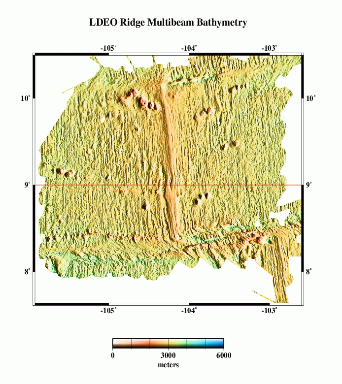 |
B | 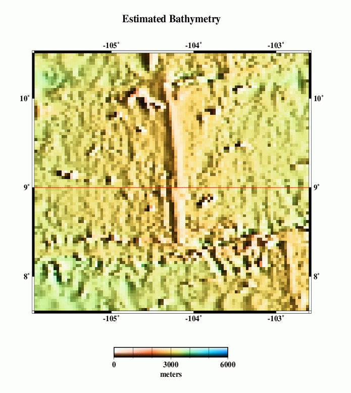 |
C | 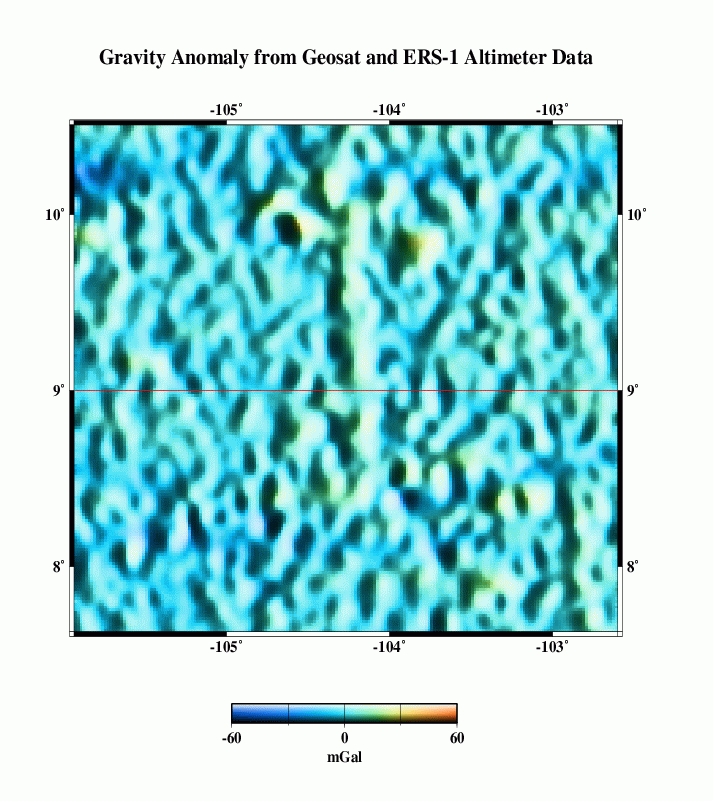 |
|---|
| D | 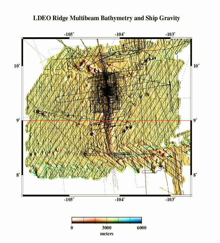 |
E | 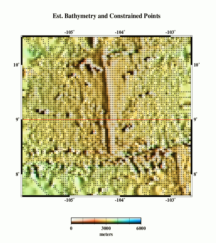 |
F | 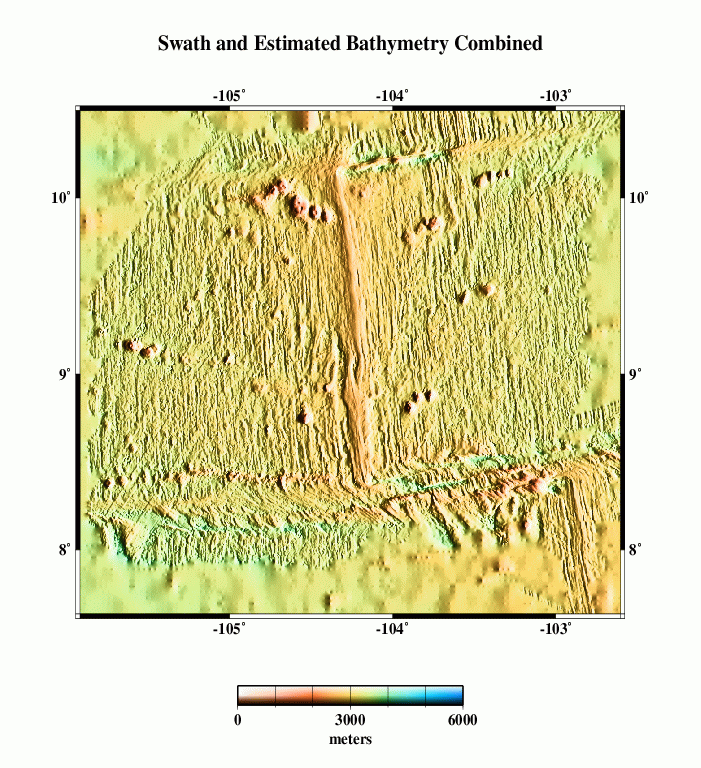 |
|---|
| G | 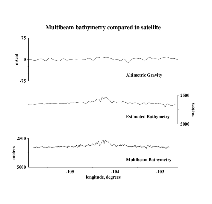 |
|---|
Grid Analysis
We compare the difference between altimetry-estimated bathymetry (2 min. grid) and actual swath bathymetry (.0028 deg. grid) two ways, because the two are on grids of different spacing and thus may capture different length scales of bathymetric roughness.
For the lower-resolution analysis (H and I), multibeam data were averaged into corresponding 2-arc-minute blocks, and estimated bathymetry was subtracted. For the higher-resolution analysis (J and K), bilinear interpolation was used to obtain estimated bathymetry values at each point on the swath bathymetry grid, then the estimated bathymetry was subtracted.
In both cases, we find the mean difference is ~ 34 m (the swath bathymetry data are systematically deeper); the difference is about 1% of the depth. An error like this is expected because of the uncertainties in whether or not data sets used in calibration have been corrected for the variable speed of sound in seawater, errors translating uncorrected sound speeds between nominal fathoms and nominal meters, etc.
The standard deviations about the mean are 71 m for the 2 arcmin averages and 82 m for the multibeam points. Since 82² - 71² ~= 41², We may assume that the root-mean-square (rms) average roughness captured by the multibeam and not capturable on a 2 arcmin grid is about 41 m. The rms difference at longer scales, 82 m, is due to incomplete information in the estimated bathymetry grid.
| H | 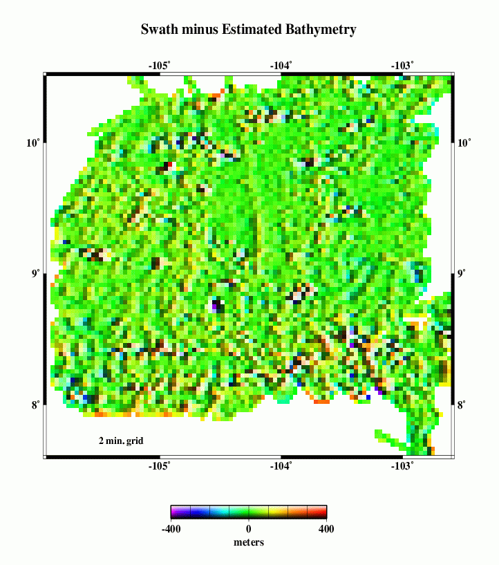 |
I | 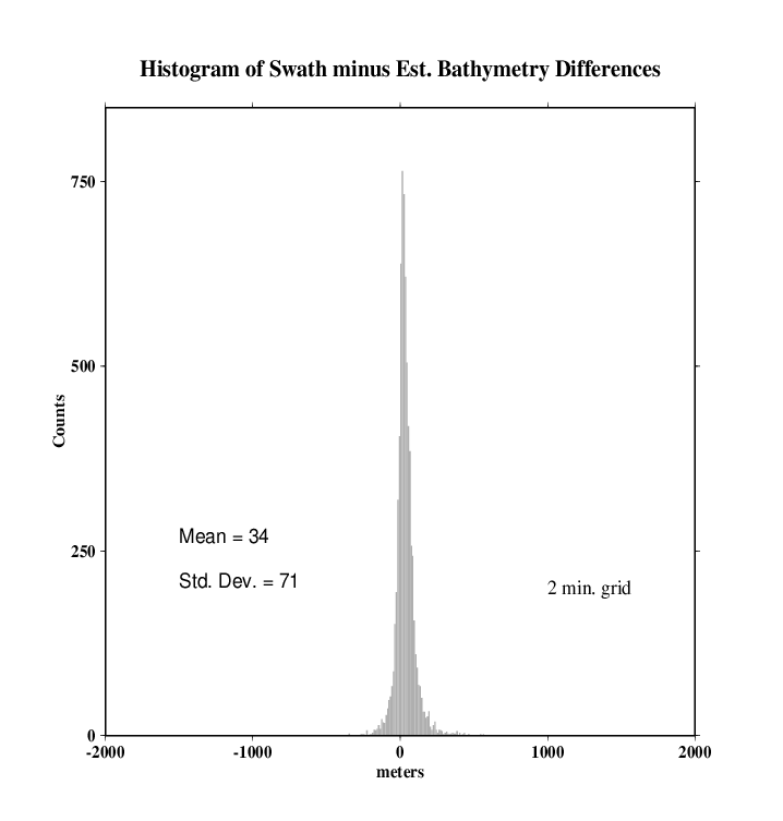 |
|---|
| J | 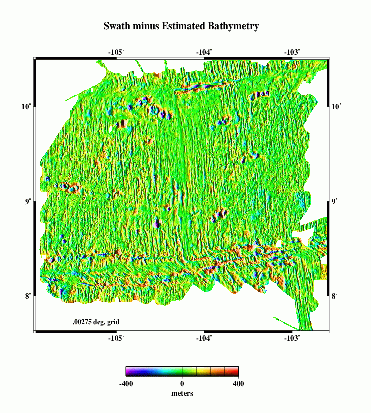 |
K | 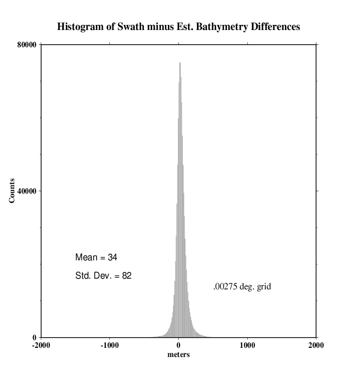 |
|---|
Eventually, we want to do a detailed cross-spectral analysis to determine how much of the actual multibeam bathymetry is captured in the altimeter gravity field. Here, we present a very simplified model. We take the combined bathymetry (F) and simply calculate a model gravity field, assuming that all the topography has the same density and is entirely uncompensated. This model (M) does not look much like the observed gravity (L), because our assumptions are too simple. The radially-averaged power spectra of the two (N) give some clue as to why.
At wavelengths longer than ~80 km or so, the simple model has too much power, because it does not include the effects of isostatic compensation of the topography. At shorter wavelenghts, the simple model also has more power, this is because at low latitudes, the nearly north-south satellite tracks do not resolve the short wavelength east-west anomalies well. We need high-quality ship gravity data to compare, such data cover only about three quarters of the study area.
| L | 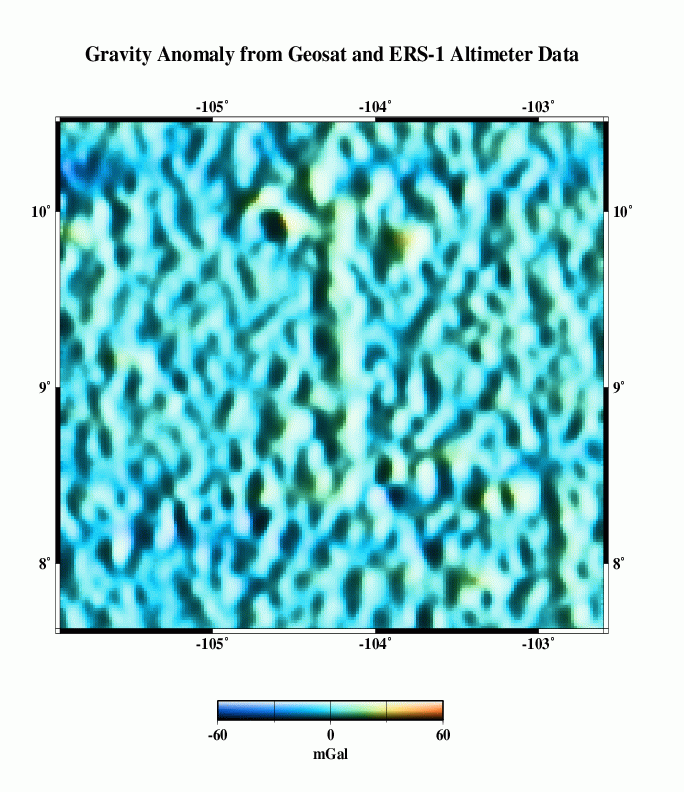 |
M | 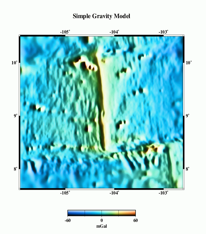 |
N | 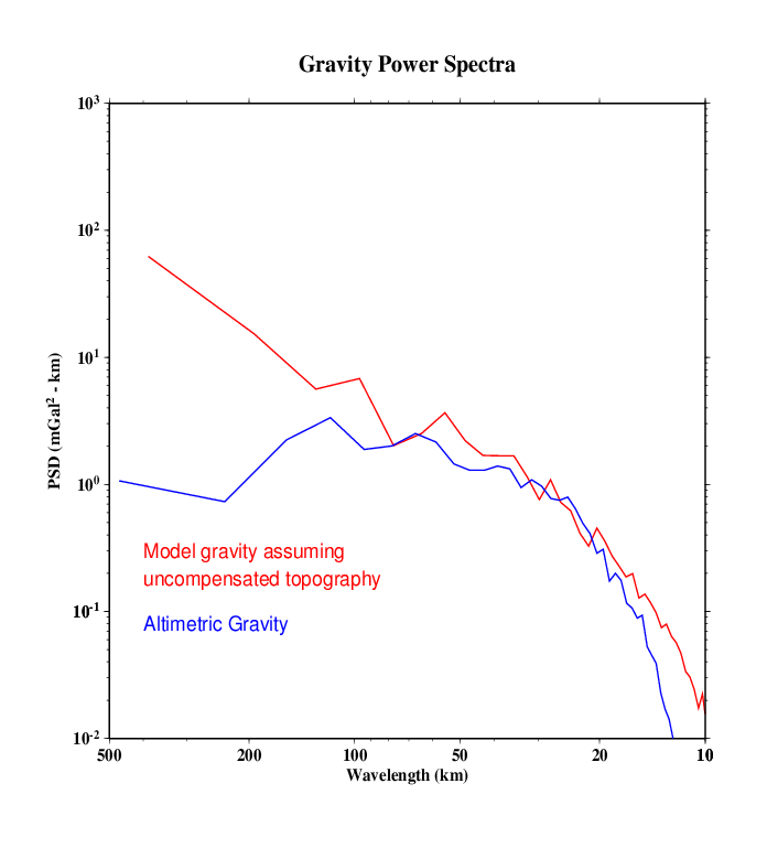 |
|---|